A Simple Project - Ethylene Oxide to Ethylene Glycol
If you have never used REX before, this quick example may be the best way to get started. Here, we illustrate the steps in estimating the kinetic model for Ethylene Oxide Hydration to Ethylene Glycol. This reaction is described in Elements of Chemical Reaction Engineering (4th Edition), H. Scott Fogler, 2005, Prentice Hall and can be built in approximately 10 minutes:
Ethylene-Oxide(ETO) + Water → Ethylene-Glycol(ETG)
The first step is to add a project. In the main Projects node, enter the new project, that we name EOEG_Example. When entering the project name, the row header icon changes from an asterisk to a pencil. Press ENTER to load the EOEG project into REX:
First, you may choose the units for the project in the Units Configuration node. We leave the default units unchanged:
Locate the Compounds node in the Project tree and enter the compounds to be used in the project. Remember to press ENTER after loading compound names to ensure that they are loaded into the REX project:
Now we go to Reactions node and enter the reaction name ETOtoETG.
Following that, we define its stoichiometry in the Stoichiometry grid located below. Note that the ETOtoETG reaction should be selected in the Reactions Grid to enter its stoichiometry:
You may have noticed the different color of the headers on the two grids of the image above.
Orange header is used for grids with independent information, like the reaction names. The Blue header on the Stoichiometry grid indicates that its information depends on the reaction chosen in the orange grid. You can find more details on the REX format in the REX Color and Caption Code section.
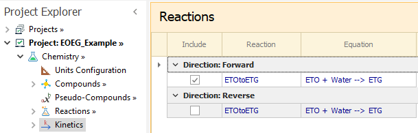
Next, we define the reaction kinetics in Chemistry → Kinetics, where we keep the default options and only Forward direction is included for this example.
We must define the initial parameter values for the reaction in the Chemistry → Kinetics → Parameters node.
We entered as initial estimates: Preexponential=0.1 and Activation Energy=0.
This reaction is order 1 with respect to ETO. We can set that by two procedures:
Having entered the Chemistry, we now proceed to the Kinetic Estimation task. In the Estimation node, we select the reactions whose parameters are to be estimated. Those reactions not marked for estimation will have their parameters fixed to the initial values loaded in Parameters node.
Here, we have only one reaction for which we estimate its parameters:
In the Estimation → Parameters node, the lower and upper bounds for the parameters are specified.
If you wish to keep the bounds close to the initial values loaded earlier, you may execute the Initialize Bounds → Current Values action, for All variables. You may also execute the Initialize Bounds → By Percent of Current action that changes the bounds by user-entered percentages with respect to the initial values.
Here, we wish to estimate only the pre-exponential value. So the bounds for the pre-exponential are manually entered in the grid as shown below. We choose to set pre-exponential lower bound to 0 and upper bound to 10; other parameters are left with closed bounds:
As for the Rate Bounds in the second tab of this node, we keep the default values +/- 1E+8, that for practical purposes implies that the reaction rate values are unbounded.
The next step is to define the reactor characteristics. Here, we model a liquid batch reactor with no inflows or outflows, where volume and temperature are Interpolated from Data:
We add just one experimental set in the Experiments node:
In Measurements node, we select the measured variables: all values for Total Moles are included for this example. Since we do not have any data for liquid Phase concentration, we do not include any compound in the liquid phase:
A new node for the experimental set just defined appears now. If you do not see the set1 node, please perform the Refresh action available through the icon in the top Toolbar.
The new node will appear with two tabs for Total Moles and Liquid, with all data as zero:
Suppose we have the initial condition for this system, plus seven measurements of ETG total moles taken at different times. In order to enter that information, we must have six additional rows to account for all time measurements. You may add them one by one by entering any variable value in the row with the (*) symbol:
A faster way is by executing the Add Datapoint action, either by right click on the set node, or through the icon in the Toolbar. This way, we can add the six additional datapoints in one step.
Now we load the experimental data, which can be done manually or by pasting from Excel if that is convenient. Here, you may manually enter the data as shown below:
Please note that the initial condition (time=0) must be specified completely for all compounds. For other points, it is not a problem if some species have no measurements. In this example, ETO and Water are not monitored, thus their unknown values will appear as zero. Regarding Volume and Temperature, because they were set as constant in Reactor node, the value entered at the initial condition is kept fixed in the model throughout the batch operation. Their values are only needed at the initial point.
As we do not have concentration measurements in the Liquid Phase, we do not enter any data in the Phase tab.
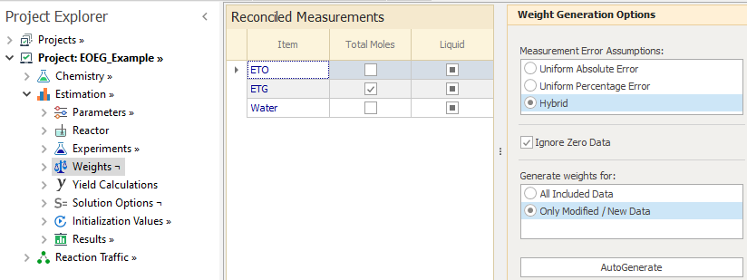
Using the experimental data, we can estimate the reaction pre-exponential by minimizing the gap between experimental and calculated ETG values using weighted least squares method. To do that, we go to Weights node and select Total Moles of ETG as a reconciled measurement. We keep the default weighting options and generate weights by pressing the Autogenerate button:
More details on the weighting options can be found in the Weights help document
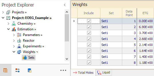
The generated weights are documented in the History tab of the node and the actual Weights values can be seen in a child node:
Then, we go to Solution Options node and choose Kinetic Parameters → Estimate, which should be enabled by default:
If you choose Kinetic Parameters → Simulate Only, the run will simulate the system using the initial estimates of the kinetics parameters as entered in the Estimation → Parameters node. Kinetic Estimation will not be performed.
Before proceeding with the run, it is always advisable to run the Check Model action to check for problems in the model specifications. You can do this in any node by first clicking in the Open Solver icon in the toolbar:
If no critical issues are detected, you may execute either the Quick Run on the toolbar or the Run that is shown after executing the Open Solver:
After the successful solution, you can inspect the solution in the Results node tree.
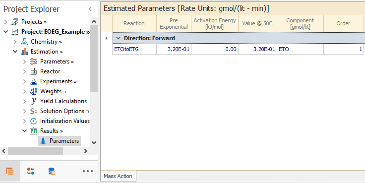
For example, in Results → Parameters node you will find the optimal values for the estimated parameters:
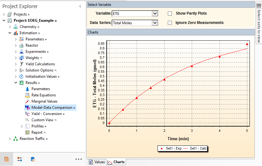
To see how the model predicts the ETG data, you can go to the Results → Model Data Comparison node:
You may explore other nodes in the tree. Help on each node can be accessed with the F1 key. You may also compare your results with the provided EOEG_Example.rex example located in the Optience Corporation\REX Suite\REX Examples folder of your installation directory.
Ethylene-Oxide(ETO) + Water → Ethylene-Glycol(ETG)
The first step is to add a project. In the main Projects node, enter the new project, that we name EOEG_Example. When entering the project name, the row header icon changes from an asterisk to a pencil. Press ENTER to load the EOEG project into REX:

|
|---|
First, you may choose the units for the project in the Units Configuration node. We leave the default units unchanged:

|
|---|
Locate the Compounds node in the Project tree and enter the compounds to be used in the project. Remember to press ENTER after loading compound names to ensure that they are loaded into the REX project:
|
|---|
Now we go to Reactions node and enter the reaction name ETOtoETG.
Following that, we define its stoichiometry in the Stoichiometry grid located below. Note that the ETOtoETG reaction should be selected in the Reactions Grid to enter its stoichiometry:
|
|---|
You may have noticed the different color of the headers on the two grids of the image above.
Orange header is used for grids with independent information, like the reaction names. The Blue header on the Stoichiometry grid indicates that its information depends on the reaction chosen in the orange grid. You can find more details on the REX format in the REX Color and Caption Code section.
Next, we define the reaction kinetics in Chemistry → Kinetics, where we keep the default options and only Forward direction is included for this example.
|
|---|
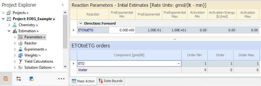
We must define the initial parameter values for the reaction in the Chemistry → Kinetics → Parameters node.
We entered as initial estimates: Preexponential=0.1 and Activation Energy=0.
This reaction is order 1 with respect to ETO. We can set that by two procedures:
- Manual entry of that order in the Orders grid
- Using the Initialize Orders action, which can be executed by right click on the node or by the icon in located the Toolbar.
After executing this action, the orders entered are the same as the reaction molecularity. Thus, it loads order 1 for both ETO and Water. We can delete the row for Water order, or reset Water order to zero. The latter is done in the view shown below:
|
|---|
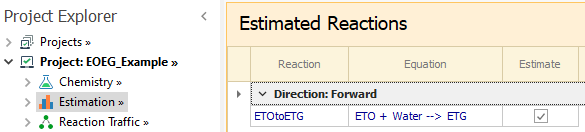
Having entered the Chemistry, we now proceed to the Kinetic Estimation task. In the Estimation node, we select the reactions whose parameters are to be estimated. Those reactions not marked for estimation will have their parameters fixed to the initial values loaded in Parameters node.
Here, we have only one reaction for which we estimate its parameters:
|
|---|
In the Estimation → Parameters node, the lower and upper bounds for the parameters are specified.
If you wish to keep the bounds close to the initial values loaded earlier, you may execute the Initialize Bounds → Current Values action, for All variables. You may also execute the Initialize Bounds → By Percent of Current action that changes the bounds by user-entered percentages with respect to the initial values.
Here, we wish to estimate only the pre-exponential value. So the bounds for the pre-exponential are manually entered in the grid as shown below. We choose to set pre-exponential lower bound to 0 and upper bound to 10; other parameters are left with closed bounds:
|
|---|
As for the Rate Bounds in the second tab of this node, we keep the default values +/- 1E+8, that for practical purposes implies that the reaction rate values are unbounded.
The next step is to define the reactor characteristics. Here, we model a liquid batch reactor with no inflows or outflows, where volume and temperature are Interpolated from Data:

|
|---|
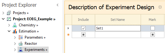
We add just one experimental set in the Experiments node:
|
|---|
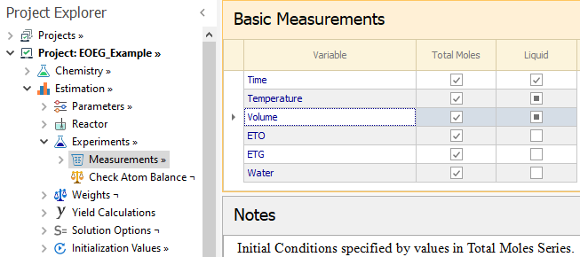
In Measurements node, we select the measured variables: all values for Total Moles are included for this example. Since we do not have any data for liquid Phase concentration, we do not include any compound in the liquid phase:
|
|---|
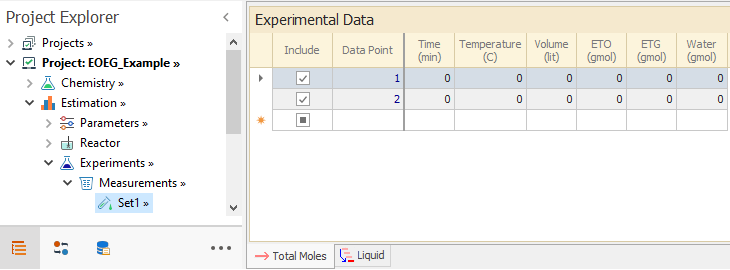
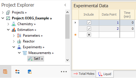
A new node for the experimental set just defined appears now. If you do not see the set1 node, please perform the Refresh action available through the
icon in the top Toolbar.The new node will appear with two tabs for Total Moles and Liquid, with all data as zero:
|
|---|
|
|---|
Suppose we have the initial condition for this system, plus seven measurements of ETG total moles taken at different times. In order to enter that information, we must have six additional rows to account for all time measurements. You may add them one by one by entering any variable value in the row with the (*) symbol:
|
|---|
A faster way is by executing the Add Datapoint action, either by right click on the set node, or through the
icon in the Toolbar. This way, we can add the six additional datapoints in one step.
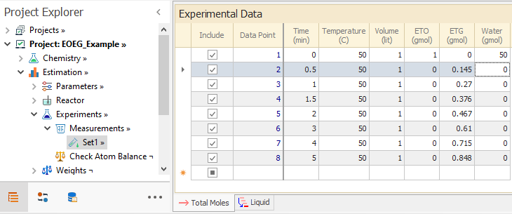
Now we load the experimental data, which can be done manually or by pasting from Excel if that is convenient. Here, you may manually enter the data as shown below:
|
|---|
Please note that the initial condition (time=0) must be specified completely for all compounds. For other points, it is not a problem if some species have no measurements. In this example, ETO and Water are not monitored, thus their unknown values will appear as zero. Regarding Volume and Temperature, because they were set as constant in Reactor node, the value entered at the initial condition is kept fixed in the model throughout the batch operation. Their values are only needed at the initial point.
As we do not have concentration measurements in the Liquid Phase, we do not enter any data in the Phase tab.
Using the experimental data, we can estimate the reaction pre-exponential by minimizing the gap between experimental and calculated ETG values using weighted least squares method. To do that, we go to Weights node and select Total Moles of ETG as a reconciled measurement. We keep the default weighting options and generate weights by pressing the Autogenerate button:
|
|---|
More details on the weighting options can be found in the Weights help document
The generated weights are documented in the History tab of the node and the actual Weights values can be seen in a child node:
|
|---|
Then, we go to Solution Options node and choose Kinetic Parameters → Estimate, which should be enabled by default:

|
|---|
If you choose Kinetic Parameters → Simulate Only, the run will simulate the system using the initial estimates of the kinetics parameters as entered in the Estimation → Parameters node. Kinetic Estimation will not be performed.
Before proceeding with the run, it is always advisable to run the Check Model action to check for problems in the model specifications. You can do this in any node by first clicking in the
Open Solver icon in the toolbar:
|
|---|
If no critical issues are detected, you may execute either the Quick Run on the toolbar or the Run that is shown after executing the Open Solver:
|
|---|
After the successful solution, you can inspect the solution in the Results node tree.
For example, in Results → Parameters node you will find the optimal values for the estimated parameters:
|
|---|
To see how the model predicts the ETG data, you can go to the Results → Model Data Comparison node:
|
|---|
You may explore other nodes in the tree. Help on each node can be accessed with the F1 key. You may also compare your results with the provided EOEG_Example.rex example located in the Optience Corporation\REX Suite\REX Examples folder of your installation directory.
Top of Topic
Go back to: