Solution Options ¬
The Solution Options Node allows you to specify strategies for the solution of the estimation problem. The choice of these options may affect the solution obtained, the robustness of the solver and the solution speed. They are explained in detail below.
Actions
Tabbed Views
Estimation Options
DAE Discretization Options
Estimation Options
In this tab, you may select some general options that affect the solver performance.
Estimation Options
Solver Options
Actions
Quick Run
Open Solver
Top of Topic
See Also:
In this tab, you may select some general options that affect the solver performance.
Grid Views
Estimation Options
Solver Options
Estimation Options
This grid is used to select options for the following items:
Top of Topic This grid is used to select options for the following items:
→ Warmstart:
The Warmstart option is used to select the initialization data for the concentration profiles. Better initialization of the profiles will result in improved robustness and speed. There are two options:
→ Kinetic Parameters
This option allows you to specify whether an estimation or simulation run is to be executed. There are two options:
→ Solver
There are two different solvers options available:
→ Negative Compositions
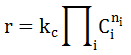
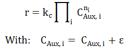
Occasionally, REX calculations may result in small negative compositions for species at intermediate solver iterations. This causes arithmetic operation errors in the reaction rate calculation, when negative concentrations are raised to a fractional exponent. For example, in the rate expression below:
If the reaction order(ni) is 0.5, and the concentration(ci) is -1e-6 mol/lit, this will result in an invalid arithmetic operation. Furthermore, even if the value of the composition is zero, the derivative of the rate equation at this point becomes infinity, because the derivative is exponentiated to -0.5. This also may cause convergence difficulties.
REX provides several options to avoid these problems which are described below.
→ Use Composition Bounds
If you choose "Yes", the bound values that you have specified for the compounds and pseudo-compounds in the Bounds node are enforced.
If you select "No", the specified values of the bounds are ignored in the model. However, please note that bounds specified for the flows which are used for pressure control in batch reactor are always honored even if you select "No".
→ Use Rate Bounds
If you choose "Yes", the bound values that are specified for the rates in the Rate Bounds tab are enforced.
If you select "No", the specified values of the bounds are ignored in the model.
→ Calculate Confidence
If you choose "Yes" and Estimate is selected in Kinetic Parameters, the Estimation run will be followed by simulations to calculate the 95% confidence interval for the kinetic parameters that were estimated.
If you select "No" and/or you choose Simulate Only for the Kinetic Parameters, the confidence interval calculations are not done.
This Example illustrates the use of this feature. As the confidence interval calculations can take significant computation time, it is advisable that you disable this option during the preliminary model development stage. After reaching a reasonably satisfactory solution, you may enable this option to estimate the confidence intervals.
The Warmstart option is used to select the initialization data for the concentration profiles. Better initialization of the profiles will result in improved robustness and speed. There are two options:
- Experimental Data (Default): REX takes the experimental data provided in the Measurements node, and initializes the concentration profiles using this experimental data. The values provided in Initialization Values are not used.
- Use Provided Initial Values: The initialization is performed with the values from Initialization Values. Here, initialization values for each state variable must be provided at each finite element and collocation point (see Finite Elements below). If you select this option, you should ensure that reasonable values are provided here, otherwise, you may have convergence problems. One way to provide reasonable values is to initialize from a previously converged solution by using the Initialize from results action in the Estimation or Initialization Values node.
→ Kinetic Parameters
This option allows you to specify whether an estimation or simulation run is to be executed. There are two options:
- Simulate Only: The kinetic parameters entered in Parameters node will be fixed, so no parameter estimation will be performed. The results will be the predicted concentrations for the parameter values, along with the experimental data.
- Estimate (Default): The kinetic parameters are optimized so that the difference between the Experimental and Calculated Values are minimized based on the Least Squares Objective Function.
→ Solver
There are two different solvers options available:
- Conopt3
- Conopt4
→ Negative Compositions
Occasionally, REX calculations may result in small negative compositions for species at intermediate solver iterations. This causes arithmetic operation errors in the reaction rate calculation, when negative concentrations are raised to a fractional exponent. For example, in the rate expression below:
|
|---|
- Force zero values - Approximate: This is the default option for a new project. The equation below illustrates the difference between this implementation and the basic rate equation above. It uses a smooth approximation of the Max function (used in the exact method listed after this option) in the rate equation for the compounds that have noninteger orders. The rate expression used here is:
where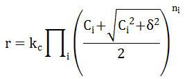
 is called the zero tolerance whose default value is 10-6. This value can be changed in the Solver Options view. Choosing a non-zero value ensures that the derivative for an exponent of 0.5 will never go to infinity.
- Force zero values - Exact: By using this option, the model uses the non-smooth function Max(0,x) in the reaction rate equation, thus avoiding problems of negative concentrations raised to a fractional order:
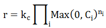
Although this implementation will avoid the problem of small negative concentration raised to noninteger orders, it has the numerical disadvantage of using the Max(0,x) function which is nondifferentiable at x=0. Furthermore, the derivative of the rate equation can go to infinity if the reaction order(ni) is less than 1. Therefore, although this is an exact implementation, the previous option that approximates the Max function may work better.
- Negative Allowed: The original rate equations are used with no modifications.
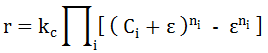
- Use Slack: A small positive tolerance
 called the slack is introduced as indicated below, to compensate for small negative concentrations:
- Use Slack - REX 2.3 method: An auxiliary variable, that includes a small positive tolerance, is used in the rates calculation:
→ Use Composition Bounds
If you choose "Yes", the bound values that you have specified for the compounds and pseudo-compounds in the Bounds node are enforced.
If you select "No", the specified values of the bounds are ignored in the model. However, please note that bounds specified for the flows which are used for pressure control in batch reactor are always honored even if you select "No".
→ Use Rate Bounds
If you choose "Yes", the bound values that are specified for the rates in the Rate Bounds tab are enforced.
If you select "No", the specified values of the bounds are ignored in the model.
→ Calculate Confidence
If you choose "Yes" and Estimate is selected in Kinetic Parameters, the Estimation run will be followed by simulations to calculate the 95% confidence interval for the kinetic parameters that were estimated.
If you select "No" and/or you choose Simulate Only for the Kinetic Parameters, the confidence interval calculations are not done.
This Example illustrates the use of this feature. As the confidence interval calculations can take significant computation time, it is advisable that you disable this option during the preliminary model development stage. After reaching a reasonably satisfactory solution, you may enable this option to estimate the confidence intervals.
Solver Options
The list of tuning options for both REX and the Nonlinear Solver are provided here. The options indicated as "For Debug Only" will not change the solver performance.
Top of Topic The list of tuning options for both REX and the Nonlinear Solver are provided here. The options indicated as "For Debug Only" will not change the solver performance.
REX Options
→ Autorun Check Model
If this is ON, Checkmodel (see Solver → CheckModel view) is first executed before running the estimation model. If there are any critical messages, the run will be cancelled. If this is OFF, the estimation run will proceed without any model checks. The default is ON (set to 1).
→ CPU Time Limit
Maximum amount of time used by the solver. Enter an integer value in seconds.
→ Detailed Solution Listing (for debug only)
This option controls the printing of the model solution in the listing file. Enter 1 for generating a detailed solution status listing file that will be saved when you choose to record an estimation or optimization run. The default value of 0 generates a compact solution status listing file.
→ Iterations Limit
It sets a limit on the number of iterations (integer) performed by the solver. If this limit is hit, the solver will terminate and return solver status 2 ITERATION INTERRUPT. The default value is 1000 iterations. You may set a higher value if the solution is not found because that limit is reached.
→ Jacobian Variables List Limit (for debug only)
This controls the number of specific variables (along with their first order Taylor coefficients) displayed for each block of variables.
→ Linearized Equations List Limit (for debug only)
This controls the number of speciifc equations (and their first order Taylor approximations) displayed for each block of equations
→ Negative Compositions -> Slack Max Definition
This option pertains to the Use Slack option for Negative Compositions. Change the default value of 0 to 1 if you would like REX to use a user-specified maximum value for the slack. The actual slack value is entered in the row below. If the default value(0) is used, REX generates an estimate of this maximum slack value automatically.
→ Negative Compositions -> Slack Max Value
The maximum value of slack can be entered here. This value is ignored if the Slack max definition in the row above is set to 0 (automatic).
→ Negative Compositions -> Zero Tolerance
The value loaded here is used only when the Force Zero - Approximate option is chosen for negative compositions. You may enter the value of the zero tolerance here.
→ Perturbation for Activation Energy
The value entered here is used only when the Confidence Calculation option is enabled. It represents the perturbation from the estimated value of Activation Energy in order to calculate the sensitivities which are needed for the confidence interval calculations. The default value is 1 kJ/mol.
→ Perturbation for Orders
The value entered here is used only when the Confidence Calculation option is enabled. It represents the perturbation from the estimated value of the compounds order to calculate the sensitivities which are needed for the confidence interval calculations. The default value is 0.01.
→ Perturbation for Preexponentials
The value entered here is used only when the Confidence Calculation option is enabled. It represents the perturbation from the estimated value of the preexponential factor in order to calculate the sensitivities which are needed for the confidence interval calculations. The default is -3%, meaning that the simulation is done by decreasing the optimal value by 3%.
→ Perturbation for Stoichiometric Coefficients
The value entered here is used only when the Confidence Calculation option is enabled together with the estimation of stoichiometric coefficients in the Estimation node. It represents the perturbation from the estimated value of the stoichiometric coefficient in order to calculate the sensitivities which are needed for the confidence interval calculations. The default is 0.01.
→ Significant Figures for Initialization Values
You may define how many significant values will be reported for the variables that are used in the initialization of future runs. In general, increased significant figures should result in better initialization. The default is 7.
→ Threads to be used by solver
This option is applicable for estimation runs with Confidence Calculation option enabled. You may set the number of simulation runs that can be done in parallel.
Default value is 0, so all available physical threads in your PC will be used. You can enter any integer value, or -1 that implies that all but one available threads in the PC will be used.
→ Threshold for point equilibrium
This is used to indicate whether the reaction can be considered as equilibriated.
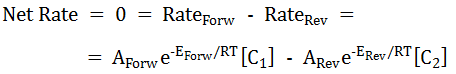
For example, consider a reaction . If this reaction were actually at equilibrium, its net rate would be zero for all sets and all points:
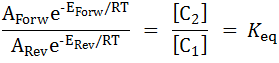
Rearranging, we have :
The last relation holds when the reaction is fast enough to be completely at equilibrium. What REX does is to count the points (N) where the relative difference between the first term and second term in the above equation is within the specified Threshold for Point equilibrium. The default value for this threshold is 2%. This is compared with the total number of points where reactor compositions are calculated (M). If 100*N/M is greater than the Threshold for Region at Equilibrium number described below, then the reaction is marked as being close to equilibriated and a flag is shown in Estimation → Results → Parameters node. The number M is equal to the total number of collocation points for Batch/PFR/Fixed Bed reactors and equal to the number of CSTRs for n-CSTR reactors. It is important to note that REX uses the compound orders at the end of the estimation/simulation run to figure out the second term in the last equation above. If the compound orders are not the same as the molecularity, then the equilibrium check will not be thermodynamically consistent.
→ Threshold for region at equilibrium
This option is to indicate whether a reaction can be considered to be at equilibrium and is explained above. The default value is 80%.
Conopt3 Options
→ Bending Line Search
(From the CONOPT documentation)
This is a method for finding the maximal step while searching for a feasible solution. The step in the Newton direction is usually either the ideal step of 1.0 or the step that will bring the first basic variable exactly to its bound. An alternative procedure uses "bending": All variables are moved a step s and the variables that are outside their bounds after this step are projected back to the bound. The step length is determined as the step where the sum of infeasibilities, computed from a linear approximation model, starts to increase again. The advantage of this method is that it often can make larger steps and therefore better reductions in the sum of infeasibilities, and it is not very sensitive to degeneracies. The alternative method is turned on by setting this to 1, and it is turned off by setting it to 0.
You may try activating this option (set to 1) when you see several solver iterations where both the MX and OK flag show equal to F. This indicates that the step search was not determined by a variable reaching a bound (MX=F), and that the line search was terminated because it was not possible to find a feasible solutions for large step lengths (OK=F).
→ Limit for slow progress (for debug only)
Limit for slow progress / no improvement. The default value is 50.
The estimation is stopped with a "Slow Progress" message if the change in objective is less than 10 * rtobjr * max(1,abs(FOBJ)) for N consecutive iterations, where N is the value entered for this option, FOBJ is the value of the current objective function, and rtobjr is the Relative objective tolerance whose default value on most machines is around 3.E-13.
→ Maximum Jacobian Tolerance
Maximum Jacobian element. The optimization is stopped if a Jacobian element exceeds this value. If you need a larger value, then your model may be poorly scaled and may be harder to solve.
→ Maximum variable
This is an internal value of infinity. The model is considered unbounded if a variable exceeds this absolute value. If you need a larger value, then your model may be poorly scaled and may be harder to solve.
→ Minimum Feasibility Tolerance
(From the CONOPT documentation)
A constraint will always be considered feasible if the residual is less than this tolerance times MaxJac, independent of the dual variable. MaxJac is an overall scaling measure for the constraints computed as max(1,maximal Jacobian element/100).
The default value is 4.E-10. You should only increase this number if you have inaccurate function values and you get an infeasible solution with a very small sum of infeasibility, or if you have very large terms in some of your constraints (in which case scaling may be more appropriate). Square systems (which result from running Simulate Only), are always solved to this tolerance.
→ Optimality Tolerance
Optimality tolerance. This is usually relevant for large models. The solution is considered optimal if the reduced gradient is less than this tolerance. If you have problems with slow progress or see small changes in the objective function through many iterations, you may increase this tolerance. The default value is 1.E-7.
→ Scaling Switch
(From the CONOPT documentation)
This is a logical switch that turns model scaling ON (Enter 1) or OFF (Enter 0). The default value is 1.
→ Slack Basis Switch
(From the CONOPT documentation)
If this option is set to ON then the first basis after preprocessing will have slacks in all infeasible constraints and Phase 0 will usually be bypassed. This is sometimes useful together with Triangular Crash Switch = ON if the number of infeasible constraints after the crash procedure is small. It is necessary to experiment with the model to determine if this option is useful. In REX, this option has been effective for systems with large degrees of freedom, such as in Pressure Controlled Reactors, where the flow is optimized at each integration point to minimize the deviation of the pressure from the set point.
→ Triangular Crash Switch
(From the CONOPT documentation)
The crash procedure tries to identify equations with a mixture of un-initialized variables and variables with initial values, and it solves the equations with respect to the un-initialized variables.
Conopt4 Options
→ Flag for pre-selecting slacks for initial basis
(From the CONOPT documentation)
When turned on CONOPT will select all infeasible slacks as the first part of the initial basis. The default value is 1.
→ Limit Iterations with Slow Progress
(From the CONOPT documentation)
The optimization is stopped if the relative change in objective is less than 3.0e-12 for the Limit of Iterations with Slow Progress. The default is 20.
→ Maximum feasibility tolerance after scaling
(From the CONOPT documentation)
The feasibility tolerance used by CONOPT is dynamic. As long as we are far from the optimal solution and make large steps it is not necessary to compute intermediate solutions very accurately. When we approach the optimum and make smaller steps we need more accuracy. This is the upper bound on the dynamic feasibility tolerance, with range: [1.e-10, 1.e-3]. Default value is 1.e-7.
→ Method used to determine the step in Phase 0
(From the CONOPT documentation)
The steplength used by the Newton process in phase 0 is computed by one of two alternative methods controlled:
Value=0 (default): The standard ratio test method known from the Simplex method. CONOPT adds small perturbations to the bounds to avoid very small pivots and improve numerical stability. Linear constraints that initially are feasible will remain feasible with this method. It is the default method for optimization models.
Value=1: A method based on bending (projecting the target values of the basic variables on the bounds) until the sum of infeasibilities is close to its minimum. Linear constraints that initially are feasible may become infeasible due to bending.
→ Minimum feasibility tolerance after scaling
(From the CONOPT documentation)
See Maximum feasibility tolerance after scaling for a discussion of the dynamic feasibility tolerances used by CONOPT.
The range for this option is [3.e-13, 1.e-5] and the defult value is 4.e-10.
→ Optimality tol for reduced gradient when feasible
(From the CONOPT documentation)
The reduced gradient is considered zero and the solution optimal if the largest superbasic component of the reduced gradient is less than this value. Range: [3.e-13, 1], default: 1.e-7.
→ Upper bound solution values and equation levels
(From the CONOPT documentation)
If the value of a variable, including the objective function value and the value of slack variables, exceeds this value then the model is considered to be unbounded and the optimization process returns the solution with the large variable flagged as unbounded. A bound cannot exceed this value. Range: [1.e5, 1.e30], default: 1.e8.
→ Autorun Check Model
If this is ON, Checkmodel (see Solver → CheckModel view) is first executed before running the estimation model. If there are any critical messages, the run will be cancelled. If this is OFF, the estimation run will proceed without any model checks. The default is ON (set to 1).
→ CPU Time Limit
Maximum amount of time used by the solver. Enter an integer value in seconds.
→ Detailed Solution Listing (for debug only)
This option controls the printing of the model solution in the listing file. Enter 1 for generating a detailed solution status listing file that will be saved when you choose to record an estimation or optimization run. The default value of 0 generates a compact solution status listing file.
→ Iterations Limit
It sets a limit on the number of iterations (integer) performed by the solver. If this limit is hit, the solver will terminate and return solver status 2 ITERATION INTERRUPT. The default value is 1000 iterations. You may set a higher value if the solution is not found because that limit is reached.
→ Jacobian Variables List Limit (for debug only)
This controls the number of specific variables (along with their first order Taylor coefficients) displayed for each block of variables.
→ Linearized Equations List Limit (for debug only)
This controls the number of speciifc equations (and their first order Taylor approximations) displayed for each block of equations
→ Negative Compositions -> Slack Max Definition
This option pertains to the Use Slack option for Negative Compositions. Change the default value of 0 to 1 if you would like REX to use a user-specified maximum value
for the slack. The actual slack value is entered in the row below. If the default value(0) is used, REX generates an estimate of this maximum slack value automatically.→ Negative Compositions -> Slack Max Value
The maximum value of slack
can be entered here. This value is ignored if the Slack max definition in the row above is set to 0 (automatic).→ Negative Compositions -> Zero Tolerance
The value loaded here is used only when the Force Zero - Approximate option is chosen for negative compositions. You may enter the value of the zero tolerance
here.
→ Perturbation for Activation Energy
The value entered here is used only when the Confidence Calculation option is enabled. It represents the perturbation from the estimated value of Activation Energy in order to calculate the sensitivities which are needed for the confidence interval calculations. The default value is 1 kJ/mol.
→ Perturbation for Orders
The value entered here is used only when the Confidence Calculation option is enabled. It represents the perturbation from the estimated value of the compounds order to calculate the sensitivities which are needed for the confidence interval calculations. The default value is 0.01.
→ Perturbation for Preexponentials
The value entered here is used only when the Confidence Calculation option is enabled. It represents the perturbation from the estimated value of the preexponential factor in order to calculate the sensitivities which are needed for the confidence interval calculations. The default is -3%, meaning that the simulation is done by decreasing the optimal value by 3%.
→ Perturbation for Stoichiometric Coefficients
The value entered here is used only when the Confidence Calculation option is enabled together with the estimation of stoichiometric coefficients in the Estimation node. It represents the perturbation from the estimated value of the stoichiometric coefficient in order to calculate the sensitivities which are needed for the confidence interval calculations. The default is 0.01.
→ Significant Figures for Initialization Values
You may define how many significant values will be reported for the variables that are used in the initialization of future runs. In general, increased significant figures should result in better initialization. The default is 7.
→ Threads to be used by solver
This option is applicable for estimation runs with Confidence Calculation option enabled. You may set the number of simulation runs that can be done in parallel.
Default value is 0, so all available physical threads in your PC will be used. You can enter any integer value, or -1 that implies that all but one available threads in the PC will be used.
→ Threshold for point equilibrium
This is used to indicate whether the reaction can be considered as equilibriated.
For example, consider a reaction
. If this reaction were actually at equilibrium, its net rate would be zero for all sets and all points:
|
|---|
Rearranging, we have :
|
|---|
The last relation holds when the reaction is fast enough to be completely at equilibrium. What REX does is to count the points (N) where the relative difference between the first term and second term in the above equation is within the specified Threshold for Point equilibrium. The default value for this threshold is 2%. This is compared with the total number of points where reactor compositions are calculated (M). If 100*N/M is greater than the Threshold for Region at Equilibrium number described below, then the reaction is marked as being close to equilibriated and a flag is shown in Estimation → Results → Parameters node. The number M is equal to the total number of collocation points for Batch/PFR/Fixed Bed reactors and equal to the number of CSTRs for n-CSTR reactors. It is important to note that REX uses the compound orders at the end of the estimation/simulation run to figure out the second term in the last equation above. If the compound orders are not the same as the molecularity, then the equilibrium check will not be thermodynamically consistent.
→ Threshold for region at equilibrium
This option is to indicate whether a reaction can be considered to be at equilibrium and is explained above. The default value is 80%.
Conopt3 Options
→ Bending Line Search
(From the CONOPT documentation)
This is a method for finding the maximal step while searching for a feasible solution. The step in the Newton direction is usually either the ideal step of 1.0 or the step that will bring the first basic variable exactly to its bound. An alternative procedure uses "bending": All variables are moved a step s and the variables that are outside their bounds after this step are projected back to the bound. The step length is determined as the step where the sum of infeasibilities, computed from a linear approximation model, starts to increase again. The advantage of this method is that it often can make larger steps and therefore better reductions in the sum of infeasibilities, and it is not very sensitive to degeneracies. The alternative method is turned on by setting this to 1, and it is turned off by setting it to 0.
You may try activating this option (set to 1) when you see several solver iterations where both the MX and OK flag show equal to F. This indicates that the step search was not determined by a variable reaching a bound (MX=F), and that the line search was terminated because it was not possible to find a feasible solutions for large step lengths (OK=F).
→ Limit for slow progress (for debug only)
Limit for slow progress / no improvement. The default value is 50.
The estimation is stopped with a "Slow Progress" message if the change in objective is less than 10 * rtobjr * max(1,abs(FOBJ)) for N consecutive iterations, where N is the value entered for this option, FOBJ is the value of the current objective function, and rtobjr is the Relative objective tolerance whose default value on most machines is around 3.E-13.
→ Maximum Jacobian Tolerance
Maximum Jacobian element. The optimization is stopped if a Jacobian element exceeds this value. If you need a larger value, then your model may be poorly scaled and may be harder to solve.
→ Maximum variable
This is an internal value of infinity. The model is considered unbounded if a variable exceeds this absolute value. If you need a larger value, then your model may be poorly scaled and may be harder to solve.
→ Minimum Feasibility Tolerance
(From the CONOPT documentation)
A constraint will always be considered feasible if the residual is less than this tolerance times MaxJac, independent of the dual variable. MaxJac is an overall scaling measure for the constraints computed as max(1,maximal Jacobian element/100).
The default value is 4.E-10. You should only increase this number if you have inaccurate function values and you get an infeasible solution with a very small sum of infeasibility, or if you have very large terms in some of your constraints (in which case scaling may be more appropriate). Square systems (which result from running Simulate Only), are always solved to this tolerance.
→ Optimality Tolerance
Optimality tolerance. This is usually relevant for large models. The solution is considered optimal if the reduced gradient is less than this tolerance. If you have problems with slow progress or see small changes in the objective function through many iterations, you may increase this tolerance. The default value is 1.E-7.
→ Scaling Switch
(From the CONOPT documentation)
This is a logical switch that turns model scaling ON (Enter 1) or OFF (Enter 0). The default value is 1.
→ Slack Basis Switch
(From the CONOPT documentation)
If this option is set to ON then the first basis after preprocessing will have slacks in all infeasible constraints and Phase 0 will usually be bypassed. This is sometimes useful together with Triangular Crash Switch = ON if the number of infeasible constraints after the crash procedure is small. It is necessary to experiment with the model to determine if this option is useful. In REX, this option has been effective for systems with large degrees of freedom, such as in Pressure Controlled Reactors, where the flow is optimized at each integration point to minimize the deviation of the pressure from the set point.
→ Triangular Crash Switch
(From the CONOPT documentation)
The crash procedure tries to identify equations with a mixture of un-initialized variables and variables with initial values, and it solves the equations with respect to the un-initialized variables.
Conopt4 Options
→ Flag for pre-selecting slacks for initial basis
(From the CONOPT documentation)
When turned on CONOPT will select all infeasible slacks as the first part of the initial basis. The default value is 1.
→ Limit Iterations with Slow Progress
(From the CONOPT documentation)
The optimization is stopped if the relative change in objective is less than 3.0e-12 for the Limit of Iterations with Slow Progress. The default is 20.
→ Maximum feasibility tolerance after scaling
(From the CONOPT documentation)
The feasibility tolerance used by CONOPT is dynamic. As long as we are far from the optimal solution and make large steps it is not necessary to compute intermediate solutions very accurately. When we approach the optimum and make smaller steps we need more accuracy. This is the upper bound on the dynamic feasibility tolerance, with range: [1.e-10, 1.e-3]. Default value is 1.e-7.
→ Method used to determine the step in Phase 0
(From the CONOPT documentation)
The steplength used by the Newton process in phase 0 is computed by one of two alternative methods controlled:
Value=0 (default): The standard ratio test method known from the Simplex method. CONOPT adds small perturbations to the bounds to avoid very small pivots and improve numerical stability. Linear constraints that initially are feasible will remain feasible with this method. It is the default method for optimization models.
Value=1: A method based on bending (projecting the target values of the basic variables on the bounds) until the sum of infeasibilities is close to its minimum. Linear constraints that initially are feasible may become infeasible due to bending.
→ Minimum feasibility tolerance after scaling
(From the CONOPT documentation)
See Maximum feasibility tolerance after scaling for a discussion of the dynamic feasibility tolerances used by CONOPT.
The range for this option is [3.e-13, 1.e-5] and the defult value is 4.e-10.
→ Optimality tol for reduced gradient when feasible
(From the CONOPT documentation)
The reduced gradient is considered zero and the solution optimal if the largest superbasic component of the reduced gradient is less than this value. Range: [3.e-13, 1], default: 1.e-7.
→ Upper bound solution values and equation levels
(From the CONOPT documentation)
If the value of a variable, including the objective function value and the value of slack variables, exceeds this value then the model is considered to be unbounded and the optimization process returns the solution with the large variable flagged as unbounded. A bound cannot exceed this value. Range: [1.e5, 1.e30], default: 1.e8.
DAE Discretization Options
This tab allows to specify options for the discretization of the Differential Algebraic Equation (DAE) system for the Batch and PFR reactors. This tab is not shown for CSTR reactor.
REX solves the differential equations using orthogonal collocation on finite elements. In general, the default finite element settings should be adequate. However, if you need to alter them, you may tune the following options for this solution method:
DAE Discretization Finite Elements
DAE Discretization Options
Finite Element Options
Top of Topic
Top of Topic This tab allows to specify options for the discretization of the Differential Algebraic Equation (DAE) system for the Batch and PFR reactors. This tab is not shown for CSTR reactor.
REX solves the differential equations using orthogonal collocation on finite elements. In general, the default finite element settings should be adequate. However, if you need to alter them, you may tune the following options for this solution method:
- Uniform Finite Element sizing or Specify sizing for Each Set. (In the Finite Element Sizing action)
- The number of finite elements (In the Number of Finite Elements option)
- The location of the finite elements (In the DAE Discretization Finite Elements grid)
- The order of Polynomial Approximation for state variables within the finite element (In the DAE Discretization Options grid - Polynomial Order Row)
- The location of the collocation points by specifying the quadrature type(In the DAE Discretization Options grid - Quadrature Roots Row)
Grid Views
DAE Discretization Finite Elements
DAE Discretization Options
Finite Element Options
DAE Discretization Finite Elements
This grid shows the distribution of the Finite Elements to be used in the DAE discretization. The end points of each finite element are shown as a cumulative percentage of the discretised variable total horizon. 5 finite elements are used by default with the cumulative end point %: 5, 15, 40, 70 and 100. The default widths therefore are 5, 10, 25, 30, and 30. You may change the distribution by editing the Cumulative End Point % column. To change the number of finite elements, use the Number of Finite Elements option. The default values for the finite element locations are provided for all finite element collection choices (ranging from 1 to 20 finite elements).
Note: If you have selected the Finite Element Sizing as Specify by Set in the Solution Options node, then you will see different widths for each set.
The selective placement of finite elements has a large impact on model accuracy. Increase the number of finite elements (each of smaller width) in regions where profile changes are expected to be large. For typical reaction systems, this is usually in the initial part of the reactor, therefore the default finite elements are spaced to be tighter in the initial part of the reactor. In regions where the reaction progress is rather small or fairly linear, you may have few (larger width) finite elements.
Top of Topic This grid shows the distribution of the Finite Elements to be used in the DAE discretization. The end points of each finite element are shown as a cumulative percentage of the discretised variable total horizon. 5 finite elements are used by default with the cumulative end point %: 5, 15, 40, 70 and 100. The default widths therefore are 5, 10, 25, 30, and 30. You may change the distribution by editing the Cumulative End Point % column. To change the number of finite elements, use the Number of Finite Elements option. The default values for the finite element locations are provided for all finite element collection choices (ranging from 1 to 20 finite elements).
Note: If you have selected the Finite Element Sizing as Specify by Set in the Solution Options node, then you will see different widths for each set.
The selective placement of finite elements has a large impact on model accuracy. Increase the number of finite elements (each of smaller width) in regions where profile changes are expected to be large. For typical reaction systems, this is usually in the initial part of the reactor, therefore the default finite elements are spaced to be tighter in the initial part of the reactor. In regions where the reaction progress is rather small or fairly linear, you may have few (larger width) finite elements.
DAE Discretization Options
The collocation points used in the discretization of the DAE are the roots of an orthogonal polynomial, shifted into every finite element. The options available in this grid are connected to the type of orthogonal polynomial and its order. The polynomial type you may select are Legendre and Radau, and the available orders are quadratic and cubic. The default value is the quadratic Radau polynomial.
You may have better accuracy by increasing the amount of collocation points, by selecting a cubic degree polynomial. However, cubic polynomials tend to have more oscillations at intermediate interpolation points. A tradeoff here is usually between the choice of more finite elements with a quadratic polynomial, versus the same number of finite elements with a cubic polynomial. Use more finite elements with quadratic orders when you see undesired oscillations. When oscillations are not a problem, you may use cubic polynomials, rather than increasing finite elements, to capture non-linear behaviour more efficiently.
Top of Topic
Finite Element Options
By executing the Split Marked action available on this grid, you can easily split one (or many) marked finite elements into two elements of equal width. The Finite Elements that are not marked will keep their original distribution.
In the Change Finite Element Number section of this grid, you can specify the Finite Element Sizing for the sets, where you have two choices:
When the Finite Elements Sizing option is Specify by Set, you may specify the number of finite elements differently for each set.
When the Reinitialize profiles option is ON and the number of finite elements is increased or decreased, an interpolation of the original initialization values is done onto the new ones, helping to keep the profiles close to the original profile. If this option is unselected and:
In general, increasing the number of finite elements from the default value increases the size of the problem and therefore the solution time and memory requirements. However, reducing the number of finite elements arbitrarily can compromise model accuracy. Ideally, you should minimize the number of finite elements as long as the accuracy is not compromised. One heuristic way to detect whether you have too many finite elements is to successively remove a finite element and check the resulting profiles. If the resulting profiles are within an acceptable tolerance of the original profiles, you may consider reducing the number of finite elements. The reverse test could be performed to check whether you have enough finite elements.
While the number of finite elements affects the model accuracy, the location pattern of the finite elements has a much higher impact. For special reactors such as differential reactors where we attempt to run low conversions (typically less than 10%), one or two finite elements may be quite sufficient.
By executing the Split Marked action available on this grid, you can easily split one (or many) marked finite elements into two elements of equal width. The Finite Elements that are not marked will keep their original distribution.
In the Change Finite Element Number section of this grid, you can specify the Finite Element Sizing for the sets, where you have two choices:
- Same for All Sets(Default): This means that the finite element distribution is the same for all sets. This option is reasonable to use when the profile curvature behavior is similar across the sets. If you have previously selected Specify by Set and change to Same for all Sets, REX will do the following:
- The amount of finite elements for all sets will be reset to the maximum finite element value among all sets(all = included + non-included).
- The cumulative end point % distribution in the DAE Discretization Finite Elements view will be set equal to the distribution of the set that had the highest number of finite elements. If there are 2 or more sets that have the same maximum number of finite elements, then the distribution used corresponds to the set with the lowest Display Order value.
- For sets with fewer finite elements than the maximum value (before the change to Same for all Sets), the data values for the additional collocation points added when switching to "Same to All Sets" will be missing(zeros) in the Initialization Values node. These zeros values could lead to numerical trouble when running the project with the "Initialize from Results" option. We recommend initializing these values manually in these cases.
- The amount of finite elements for all sets will be reset to the maximum finite element value among all sets(all = included + non-included).
- Specify by Set: Here, you may specify the number of finite elements for each set independently. This option is useful when the profile behavior is significantly different between the sets. If you have previously selected Same for All Sets and change to Specify by Set, REX will do the following:
- Both the amount of finite elements and the cumulative end point % in the DAE Discretization Finite Elements view will be preserved for all sets.
- You will be allowed to modify the finite element number and/or the cumulative end point % for every set.
- Both the amount of finite elements and the cumulative end point % in the DAE Discretization Finite Elements view will be preserved for all sets.
When the Finite Elements Sizing option is Specify by Set, you may specify the number of finite elements differently for each set.
When the Reinitialize profiles option is ON and the number of finite elements is increased or decreased, an interpolation of the original initialization values is done onto the new ones, helping to keep the profiles close to the original profile. If this option is unselected and:
- You increase the number of finite elements - The original points will remain unchanged while the new ones will all have zero values.
- You decrease the number of finite elements - No changes are done.
In general, increasing the number of finite elements from the default value increases the size of the problem and therefore the solution time and memory requirements. However, reducing the number of finite elements arbitrarily can compromise model accuracy. Ideally, you should minimize the number of finite elements as long as the accuracy is not compromised. One heuristic way to detect whether you have too many finite elements is to successively remove a finite element and check the resulting profiles. If the resulting profiles are within an acceptable tolerance of the original profiles, you may consider reducing the number of finite elements. The reverse test could be performed to check whether you have enough finite elements.
While the number of finite elements affects the model accuracy, the location pattern of the finite elements has a much higher impact. For special reactors such as differential reactors where we attempt to run low conversions (typically less than 10%), one or two finite elements may be quite sufficient.
Actions
Quick Run
Open Solver
Top of Topic
See Also: